MODELING OF HARMONIC NETWORK IMPEDANCE
USING EXPERIMENTAL IDENTIFICATION METHODS
Author: Eduardo Lucero
- Keywords:Modeling, Distribution and Transmission Networks, Harmonics, Signal Processing, Time Domain Parametric Methods
- ABSTRACT
- The frecuency dependent equivalent network impedance is obtained using an experimental identification methodology, based on time domain analysis of a single-input single-output system. The data used in the model development were actual recorded data, obtained during normal operating and capacitor switching conditions. The method was applied to identify the equivalent network impedance at the Alto Jahuel 66 KV substation (Endesa, Chile). The experimental conditions for the input and output signals are described. The impedance transfer function parameters are estimated considering a complete model structure for the system and the noise signal. The model is validated using non parametric methods and data from different operating conditions.
- INTRODUCTION
- The study of harmonic network impedance arises from the increasing concern about power system distortion, due to applications of power electronic devices, increasing application of shunt capacitor banks with potential for resonance conditions and decreased margins in equipment design.
- The aim of experimental identification is to develop a mathematical model wich describes the static and dynamic behavior of the system from measured input and output signals, in a sufficiently accurate manner.
- Signal processing techniques have been applied to modeling loads and radial networks, using non parametric methods based on frecuency-domain analysis [1]. Time-domain analysis has been used to identify parametric models of a distribution or transmission network [2].
- This work reports a time domain parametric method, based in an extended auto-regressive, moving-average model (ARMAX) of a single-input single-output system (SISO). The single phase Thévenin equivalent network parameters are estimated using least-squares to minimize the prediction error of a complete model structure for the system and the noise signal.
- The measurements were made using a PC personal computer with a 12 bit A/D converter, model DT 2801-A, with 8 differentials channels and a global conversion rate of 27.5 Khz [3]. The voltage record was taken from the secondary of the bus potential transformer and the current record from the line current transformer. Isolation transformers and a shunt resistance were used to adequate signals values. The analysis was performed in the same computer using the commercially available software PC-MATLAB [4].
- THEORETICAL BACKGROUND
- The problem of system identification can be described by the block diagram shown in fig.1. The principal identification procedure [5] is obtained by a comparison of the system output y and the model output ym, when the system and the model are both excited by the same input signal u. The measurable system output y consist of the unmeasurable output signal ys and the noise rs.
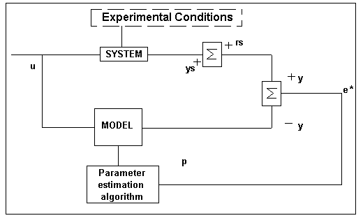 Figura Nş1: Principal Identification Procedure
- When the output signal error *e is minimal, the model becomes a candidate for modeling the system. The identification procedure can be divided into the following steps:
- planning and analyzing the experimental conditions
- selection of a rough model structure
- estimation of parameters
- model validation
- Model structure
- It is well known that a linear, time invariant, causal system can be described by its impulse response
 : :
 Ecuación Nş1
- Though most processes are of continuous type, it is advantageous to choose a discrete time model structure, compatible for parameter estimation simulation using digital computers. Assuming a sampling interval of one time unit:
 Ecuación Nş2
- introducing the backward shift operator
 , we can write: , we can write:
 Ecuación Nş3 y Nş4
- where we used the notation:
 and call G(q) the transfer operator or transfer function of the linear system [2]. and call G(q) the transfer operator or transfer function of the linear system [2].
- The output error signal according to fig.1 is:
 Ecuación Nş5
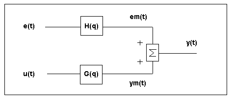
- and only vanishes for the adapted model only if an additional model for the noise signal is used, such that the complete model structure is that of fig.2.
- In this structure, it is assumed that the noise signal em(t) can be reduced to white noise e(t) by appropriate filtering using the noise filter transfer function H(q).
- If the input and output signals contain non measurable noise, then the disturbance signal has to be analyzed, considering:
- type of the signal and its frecuency spectrum
- magnitude of the disturbance
- statistic independence
- stationarity of the disturbance signal
 Figura Nş2: Complete model structure for the system and the noisy signal
- Non Parametric Methods
- It is possible to estimate the functions G and H by direct techniques without first selecting a set of possible models, using transient response analysis and correlation analysis. There are frecuency domain techniques, such as the empirical transfer function estimate using Fourier analysis and the spectral analysis. These methods are applicable for open-loop systems and cannot be applied in a straightforward fashion to closed-loop data (6).
- Parameter Estimation Methods
- To be able to estimate the functions G and H they have to be parametrized as rational functions in the delay operator
 . Assuming a basic input-output configuration as depicted in fig.2, we can write (7): . Assuming a basic input-output configuration as depicted in fig.2, we can write (7):
 Ecuación Nş7
- A much used parametric model is the extended auto-regressive (ARX) that corresponds to:
 Ecuación Nş8, 9 y 10
- the numbers na and nb are the orders of the respective polynomials, nk is the number of delays from input to output.
- Another very common model structure is the extended auto-regressive, moving average model (ARMAX):
 Ecuación Nş11 y 12
- The prediction error corresponding to (7) can be computed having observed input-output data:
 Ecuación Nş13
- The parametric identification method determines estimates of G and H by minimizing the quadratic norm
 Ecuación Nş14
- MODELING OF THE NETWORK EQUIVALENT
- The main purpose of this work is to evaluate the feasibility of obtaining accurate low-order models of the network equivalent, wich could be used for harmonic analysis and transient studies.
- Model structure
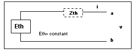
- The single phase equivalent parameters of a balanced network consisting of linear components can be deduced from the voltage and current changes consequent to a load variation caused at a node (Thévenin-Helmholtz theorem, fig.3), assuming that the interval voltage sources do not change during a measurement time of a few cycles.
 Figura Nş3
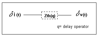
- Figure 4 shows the model structure of a SISO model, considering the current change as the input and the voltage variation as the output.
 Figura Nş4: SISO Model
- Similarly, the parameters of the other two phases are obtained and compared to validate the assumption of balanced three phase system. An alternative approach is to consider positive sequence components of the voltage and current changes.
- Otherwise the identification of the three phase matrix transfer function is a much more difficult structural problem and further development and testing is required.
- Experimental Arrangement
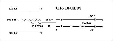
- The three phase to earth voltages and three phase currents generated by switching a 66 KV capacitor bank were recorded during a transient period before and after the switching. The measuring arrangement is shown in the one line diagram of fig.5.
 Figura Nş5
- donde:
- i, v : current, voltage measurement
- Y : star connected winding (grounded)
- D : delta connected winding
- B51: capacitor bank, 33 MVAR (ungrounded)
- B52: capacitor bank, 26.4 MVAR (ungrounded)
- Only capacitor bank B51 has a fixed reactor to limit the shunt capacitor inrush current.
- Each three phase magnitude (i,v) was recorded over a time period of 1 second before and 5 seconds after switching, digitized and stored at a conversion rate of 3440 Hz.
- EQUIVALENT NETWORK PARAMETERS
- Identification
- We assume a linear response under conditions of different frecuencies and high levels of input-output. A first order model is selected to simplify the physical interpretation of the parameters and to be consistent with the relative low dynamic range of the A/D converter. Considering a series R, L circuit:
 Ecuación Nş16
- introducing the operator p=d/dt and rearranging:
 Ecuación Nş17
- In terms of a single input (v) and a single output (i):
 Ecuación Nş18
- with
 Ecuación Nş19
- considering a delay of one unit of time (p=q-1), it is possible to write:
 Ecuación Nş20
- with
 Ecuación Nş21 y 22
- Note a different time scale in equation 17, where p=(q-1)/ep, ep=scan time interval.
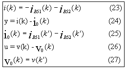
- In terms of the recorded magnitudes v(k), iB51(k), iB52(k) and the initial conditions before the switching vo(k) and io(k):
 Ecuación Nş23 a 27
- Assuming that the interval voltage sources do not change during a measurement time of a few cycles, then K`=K-nT, with T=time period of the initial condition signals, approximately 20 ms. The exact value is obtained using filtered zero crossing analysis.
- Estimation
- The problem is to calculate the coefficients of the polynomials A(q), B(q) and C(q). The polynomial coefficients and the parameters obtained using ARX and ARMAX models are listed in Table Nş1. The final prediction error (Akaikes`s FPE) and the standard deviation (x) are also indicated.
- Note that each model comes with an estimate of its own uncertainty. The relative high series resistance value (1-3 ohm) accounts for losses in the system due to high inrush currents and voltages.
- Figure 6 (phase 2) show the results corresponding to models ARX and ARMAX. The following information is presented:
- The actual response and the simulated output, considering an ideal model without noise.
- Residuals between model and actual output.
- Frecuency response of the network equivalent obtained by a non-parametric spectral analysis method compared to the model response.
TABLE Nş1: NETWORK PARAMETERS (series R, L)
| Model | FPE | b1 ± x | b2 ± x | a1 ± x | R (ohm) | L (mHy) |
ARX (120),
(phase 1) | .02866
- |
- .0061
±.0050 | .0477
± .0050 |
-.8778
±.0198 | 2.6
± 0.3 |
6.1
0.6 |
ARX (1250),
(phase 1) | .00049
- |
- .0036
±.0016 | .0445
± .0014 |
-.9142
±.0108 | 1.9
± 0.1 |
6.5
0.2 |
ARX (120),
(phase 2) | .01424
- |
- .0077
±.0116 | .0481
± .0117 |
-.8909
±.0272 | 2.3
± 0.6 |
6.0
1.5 |
ARMAX (1250),
(phase 2) | .00009
- |
- .0076
±.0020 | .0319
± .0019 |
-.9523
±.0086 | 1.5
± 0.1 |
9.1
0.5 |
- Nota:
- ARX (ijk): i=order of A(q), j=order of B(q), k=dela
- ARMAX(ijlk): .......l=order of C(q) (noise model)
- Model Validation
- The ARX (120) model testing of the residuals for independence of past inputs and whiteness is carried out in fig.7. There is a significant cross-correlation between residuals and input.
- The ARMAX (1250) model testing shows that the residuals are quite small compared to the signal level of the output (fig. 6d,c), that they are reasonably (although not perfectly) well uncorrelated with the input and between themselves, within the 95 percent confidence levels (fig.7). We can thus be satisfied with the model ARMAX (1250).
- The transient records of voltage and current initiated by energizing capacitor bank B51 are shown in fig. 8a,b (bank B52 was already connected). Note a natural frecuency

of about 170 Hz and high current values due to the energization of the capacitor bank. A different data set, from switching the other capacitor bank (B52), is used as a reference set for validation purposes (fig. 8c,d): the selected model output is compared with the actual record (fig. 8e) to verify the model is capable to reproduce the reference data set. Note time scale and signal level are very different between data sets used for estimation and validation.
- EQUIVALENT CAPACITOR BANK PARAMETERS
- The currents iB52 and iB51 were recorded separately to identify the corresponding models of the capacitor bank (first order model) and capacitor plus reactor bank (second order model). The nominal parameters provided by the manufacturers and the estimated ones were compared to validate the overall procedure, from experiment design to model estimation. The results are presented in Table Nş2.
- The parameters where obtained using different structures for the system and the noisy signal. The results for the ARX (220) and ARMAX (2250) second order models of bank B51 are shown in fig.9.
TABLE Nş2: CAPACITOR BANK PARAMETERS
| B51: R, L, C Model | R (ohm) | L (mHy) |
C (microFa) |
| ARX (220) | 13.0 ± 0.8 | 27.0 ± 0.5 |
24.0 ± 1.7 |
| ARMAX (2250) | 12.0 ± 0.1 | 26.0 ± 0.1 |
24.0 ± 0.2 |
| NOMINAL | n.a | 25.2 | 24.1 |
| B52: R,C Model | R (ohm) | - | C (microFa) |
| ARMAX (1250) | 13.5 ± 0.1 | - |
19.4 ± 0.1 |
| NOMINAL | n.a | - | 19.3 |
- CONCLUSIONS
- An application of the experimental identification methodology to the modeling of network equivalents, based on time domain analysis of a gray box single-input single-output system is reported. The impedance transfer function parameters are estimated using actual recorded data, considering a complete model structure for the system and the noise signal. Different models structure are considered and validated comparing non parametric spectral analysis estimates and testing whiteness residuals and independence between residuals and past inputs.
- The identification method is very powerful and can be used to identify other system components. The experimental procedure utilizes equipment and conditions already existing on the system. The ideal situations are capacitor/reactor switching and line energization.
- The method was applied to identify the equivalent network impedance at the Alto Jahuel 66 KV substation. The models of two capacitor banks were also identified and compared with nominal parameters provided by the manufacturers. In all cases simple linear models give a good description of the physical system. The models were essential for harmonics studies required to explain and solve a resonant condition between the network and the capacitor banks.
- Low order models were selected to simplify the physical interpretation of the parameters. By using higher order models it would be possible to adjust, almost perfectly, the model and the actual outputs. However there are other aspects to be first considered, such as the data acquisition system dynamic range. Also, the modeling of non linear time varying components and three phase systems, normally unbalanced at high frequencies, require further development and testing.
-
ACKNOWLEDGEMENTS
- The author wishes to acknowledge the efforts of Mr. Alfredo De La Quintana and Daniel Cortés of the Laboratory Division of ENDESA in carrying out the tests and making the data available. Special thanks are also extended to Prof. Alfredo Muńoz for their invaluable comments and suggestions. The author also wishes to thank Dr. Hugh Rudnick for his encouragement and helpful comments in the preparation of the paper.
- REFERENCES
- A. S. Morched, P. Kundur, "Identification and Modeling of Load Characteristics at High Frequencies", IEEE Trans. on Power Systems, Vol PWRS-2, No. 1, February 1987.
- A. A. Girgis, Jun Qiu, R. B. McManis, "A Time Domain Approach for Distribution and Transmission Network Modeling", IEEE Trans. on Power Delivery, Vol. 5, No. 1, January 1990.
- E. Lucero, L. Tapia, "Sistema portátil de medición y registro basado en un computador personal", Proceedings 7th Chilean Electrical Engineering Congress", Santiago, Chile, Noviembre, 1987.
- C. Moler, J. Little, S. Bangert, "PC-MATLAB", The Mathworks, Inc. Sherborn, Mass.
- H. Unbehauen, "System Identification Methods using Parameter Estimation / A survey", 2nd International Symposium on Systems Analysis and Simulation, Berlin, DDR, August, 1985.
- L. Ljung, "System Identification, Theory for the User", Prentice Hall, Inc. Englewood Cliffs, New Jersey.
- L. Ljung, "Identification Toolbox User's Guide", The Mathworks, Inc. Sherborn, Mass.
Volver Capacitación
Volver entrada
|


 :
:

 , we can write:
 and call G(q) the transfer operator or transfer function of the linear system [2].
